How about keeping the boring data and spreadsheet combination aside and doing something fun? I say let’s make a dice, cool? Don’t believe me? Check out this file. Keep pressing the F9 key once you’ve opened it. Magic!

Well it’s no magic, it’s fairly simple and is pure logic. I’m assuming you have some basic knowledge about Microsoft Excel and even if you don’t, no worries, I’ll teach you everything you need to know.
MS Excel cool trick: Make a dice
1. A die is a 3X3 square. Let’s begin by selecting cells C1 to I3. Cells C1 to E3 are for die 1, in between we leave a column and again cells G1 to I3 are for the second die. Next click on Format under the Home tab and select Row Height and enter 40. Again go to the Format option and click on Column Width and enter 8.
2. Now whilst the cells are still selected, choose ‘Wingdings’ as the font and set the font size to 28 and set the alignment to ‘Center’.
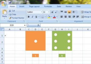
3. Once you’re done with the above steps, select cells D1 to E3 and choose any Fill Colour you desire. Do the same for cells G1 to I3.
4. To randomize the numbers of the dice, we’ll be using a function called RANDBETWEEN. The RANDBETWEEN function enables you to present random integers in a cell by pressing the F9 key. Select cell D5 and go to Formulas tab > Math & Trig and click on RANDBETWEEN. A box will pop up asking you to feed the values. Put ’1′ as the Bottom value and ’6″ as the Top value.
Select cell H5 and again use the RANDBETWEEN function and enter the same values as above.
5. Now comes the main part – using the IF function. Basically the IF function allows you to specify a condition. If the condition is true, a certain thing will happen and if false then something else will happen. For example, IF the random value in cell D5 is 3, then 3 dots will be shown on the die and if it’s 4, then 4 dots will be shown. Simple!
In cell C1 enter the following:
=IF(AND(D5>=2, D5<=6), “l”, ” “)
Now let me explain it to you how it works. The above IF condition states that if the value of the cell D5 (the random value cell) is greater than 2 but less than 6, then the outcome will be “l”, and if false, then it should be blank.
You must be wondering why the “l”? Well in the ‘Wingdings’ font the letter ‘l’ (lower case) is a dot. OMG that’s what we need, right?
In cells C2 and E2 enter the following:
=IF(D5=6,”l”, ” “)
Let’s fill up the last cell now, ie. D2:
=IF(OR(D5=1, D5=3, D5=5), “l”, ” “)
That’s it! Keep pressing the F9 key and you’ll get to know what a wonderful thing you’ve made.
As for the other die, you have to put the same formulae in the corresponding cells, the only change being ‘D5‘ replaced by ‘H5‘ in each formula.
I hope you like this stuff. It’s cool, isn’t it?